# Partial Differential Equation
Partial differential equations are defines when two or more partial derivatives are present in an equation. Due to the widespread application in engineering, we will be looking at **second-order equations** which can be expressed in the following general form:
$$
A\frac{\partial^2u}{\partial x^2} +
B\frac{\partial^2u}{\partial x \partial y} +
C\frac{\partial^2u}{\partial y^2} +
D
= 0
$$
where $A$, $B$ and $C$ are functions of both $x$ and $y$. $D$ is a a function of $x$, $y$, $u$, $\partial u / \partial x$, and $\partial u / \partial y$. Similar to our beloved quadratic formula, we can take the discriminant of the equation
$$
\Delta = B^2 - 4 AC
$$
Based on the discriminant we can categorize the equations into the following three categories:
| $\Delta$ | Category | Example |
| -------- | ---------- | ------------------------ |
| - | Elliptical | Laplace equation |
| 0 | Parabolic | Heat Conduction equation |
| + | Hyperbolic | Wave equation |
## Finite Difference Methods
### Elliptic Equations
- Used for steady-state, boundary value problems
- Examples where fields where these equations are used are: steady-state heat conduction, electrostatics and potential flow
Description of how the Laplace equations works
$$
\frac{\partial^2T}{\partial x^2}+\frac{\partial^2T}{\partial y^2}=0
$$
Finite-different solutions
- Laplacian Difference equations in dimension $x$ and $y$:
$$
\boxed{\frac{\partial^2T}{\partial x^2}= \frac{T_{i+1,j}-2T_{i,j}+T_{i-1,j}}{\Delta x^2}}
$$
$$
\frac{\partial^2T}{\partial y^2}= \frac{T_{i+1,j}-2T_{i,j}+T_{i-1,j}}{\Delta y^2}
$$
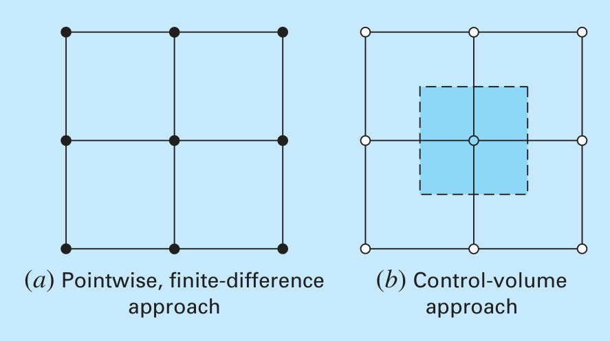
Boundary Conditions
Control-Volume approach
 Computer Algorithms
### Parabolic Equations
- Used for unstead-state, initial + boundary conditions problems
For parabolic PDE equations we also consider the change in time as well as space.
Heat-conduction equation
Explanation of heat equation
$$
k\frac{\partial^2T}{\partial x^2}=\frac{\partial T}{\partial t}
$$
Explicit methods
Forward-time central-space (FTCS Scheme)
based on forward euler method and central difference in space.
One dimensional Heat conduction example
We need to measure the insulation of a wall and measure the change of temperature through the
Simple Implicit methods
Crank-Nicolson
ADI
### Hyperbolic Equations
MacCormack Method
In computational fluid dynamics (CFD), the governing equations are the Navier-Stokes equations. For inviscid (no viscosity) compressible flow, these reduce to the Euler equations:
$$
\frac{\partial u}{\partial t}+\frac{\partial f(u)}{\partial x} = 0
$$
where, $U$ is conserved variables. This equation is a hyperbolic PDE.
Discretize domain: space and time
Write fluxes:
MacCormack Algorithm
- Predictor
$$
u^p_i = u^n_i - \frac{\Delta t}{\Delta x}(f^n_{i+1}-f^n_i)
$$
- Corrector
$$
u^{p+1}_i = \frac{1}{2}(u^n_i+u^p_i) - \frac{\Delta t}{2\Delta x}(f^p_{i}-f^n_{i-1})
$$
Method of characteristics
## Finite-Element Method
General Approach
1. Discretization
2. Element Equations
3. Assembly
4. Boundary Conditions
5. Solutions
6. Post-processing
### One-dimensional analysis
### Two-dimensional Analysis
## Problem 1: Finite-Element Solution of a Series of Springs
Problem 32.4 from Numerical Methods for Engineers 7th Edition Steven C. Chapra and Raymond P. Canale
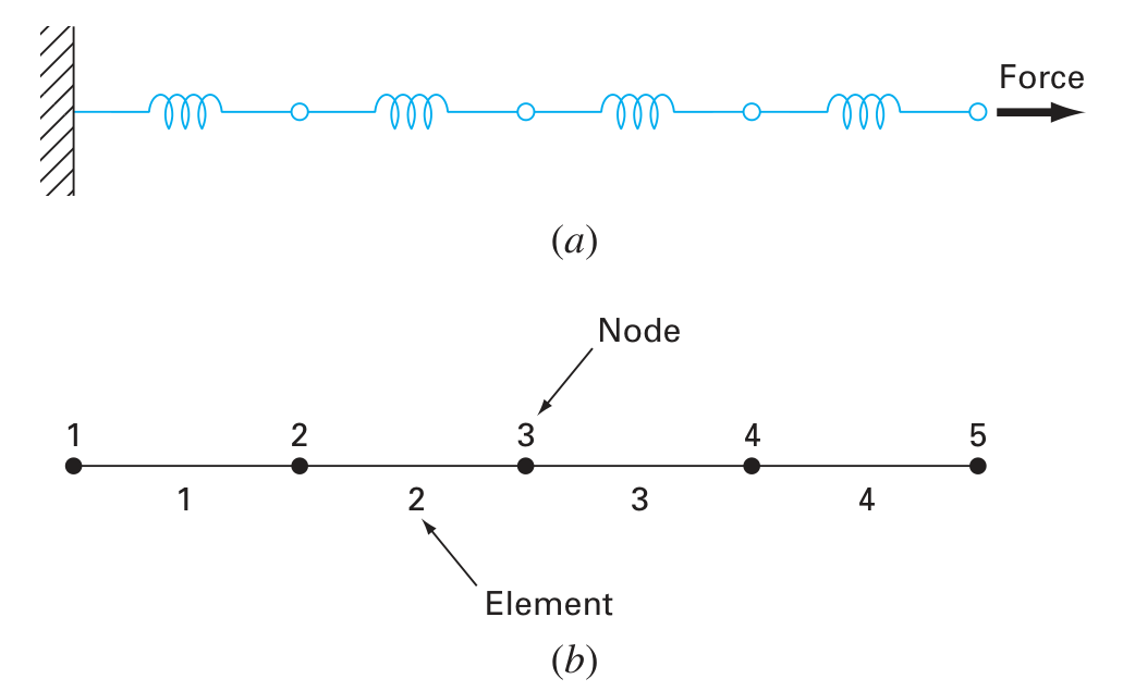
A series of interconnected strings are connected to a fixed wall where the other is subject to a constant force F. Using the step-by-step procedure from above, determine the displacement of the springs.
Solution:
Setup: Let's partition the system to treat each spring as an element. Thus, the system consists for 4 elements and 5 nodes.
Computer Algorithms
### Parabolic Equations
- Used for unstead-state, initial + boundary conditions problems
For parabolic PDE equations we also consider the change in time as well as space.
Heat-conduction equation
Explanation of heat equation
$$
k\frac{\partial^2T}{\partial x^2}=\frac{\partial T}{\partial t}
$$
Explicit methods
Forward-time central-space (FTCS Scheme)
based on forward euler method and central difference in space.
One dimensional Heat conduction example
We need to measure the insulation of a wall and measure the change of temperature through the
Simple Implicit methods
Crank-Nicolson
ADI
### Hyperbolic Equations
MacCormack Method
In computational fluid dynamics (CFD), the governing equations are the Navier-Stokes equations. For inviscid (no viscosity) compressible flow, these reduce to the Euler equations:
$$
\frac{\partial u}{\partial t}+\frac{\partial f(u)}{\partial x} = 0
$$
where, $U$ is conserved variables. This equation is a hyperbolic PDE.
Discretize domain: space and time
Write fluxes:
MacCormack Algorithm
- Predictor
$$
u^p_i = u^n_i - \frac{\Delta t}{\Delta x}(f^n_{i+1}-f^n_i)
$$
- Corrector
$$
u^{p+1}_i = \frac{1}{2}(u^n_i+u^p_i) - \frac{\Delta t}{2\Delta x}(f^p_{i}-f^n_{i-1})
$$
Method of characteristics
## Finite-Element Method
General Approach
1. Discretization
2. Element Equations
3. Assembly
4. Boundary Conditions
5. Solutions
6. Post-processing
### One-dimensional analysis
### Two-dimensional Analysis
## Problem 1: Finite-Element Solution of a Series of Springs
Problem 32.4 from Numerical Methods for Engineers 7th Edition Steven C. Chapra and Raymond P. Canale
A series of interconnected strings are connected to a fixed wall where the other is subject to a constant force F. Using the step-by-step procedure from above, determine the displacement of the springs.
Solution:
Setup: Let's partition the system to treat each spring as an element. Thus, the system consists for 4 elements and 5 nodes.
 Element Equations: Analyzing element 1 we get the following free body diagram:
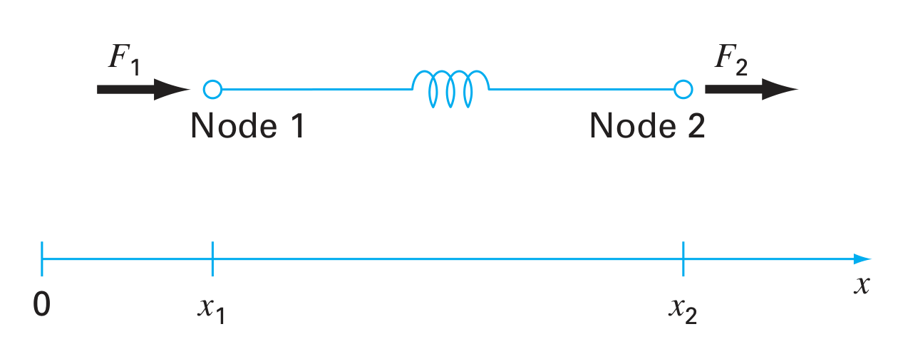 Applying Hook's law to the element we get:
$$
F=kx
$$
$$
F=k(x_1-x_2)
$$
where $(x_1-x_2)$ is how much the first spring is stretched out.
Re-writing this equation:
$$
F_1 = kx_1 - kx_2
$$
$$
F_2=-kx_1+kx_2
$$
$$
\begin{bmatrix} k & -k \\ -k & k \end{bmatrix}
\begin{Bmatrix} x_{1} \\
x_{2} \end{Bmatrix}
=
\begin{Bmatrix} F_{1} \\ F_{2} \end{Bmatrix}
$$
$$
[k]\{x\}=\{F\}
$$
where $[k]$ is the element property matrix or in this case element stiffness matrix. $x$ is a column vector of unknowns (in this case position of each) and $F$ is a vector column with external influence applied at the nodes.
Assembly: Once individual element equations are derived we will link them together using assembly.
$$
[k]\{x'\}=\{F'\}
$$
where $[k]$ is the assemblage property matrix and $\{u'\}$ and $\{F'\}$ column vectors are unknowns and external forces that are marked with primes to denote that they are an assemblage of the vectors $\{u\}$ and $\{F\}$.
$$
\begin{bmatrix} k & -k \\ -k & k \end{bmatrix}
\begin{Bmatrix} x_{1} \\ x_2 \end{Bmatrix}
$$
## Problem 2: Finite
Solve the non-dimensional transient heat conduction equation in two dimensions, which represents the transient temperature distribution in an insulated plate
---
Applying Hook's law to the element we get:
$$
F=kx
$$
$$
F=k(x_1-x_2)
$$
where $(x_1-x_2)$ is how much the first spring is stretched out.
Re-writing this equation:
$$
F_1 = kx_1 - kx_2
$$
$$
F_2=-kx_1+kx_2
$$
$$
\begin{bmatrix} k & -k \\ -k & k \end{bmatrix}
\begin{Bmatrix} x_{1} \\
x_{2} \end{Bmatrix}
=
\begin{Bmatrix} F_{1} \\ F_{2} \end{Bmatrix}
$$
$$
[k]\{x\}=\{F\}
$$
where $[k]$ is the element property matrix or in this case element stiffness matrix. $x$ is a column vector of unknowns (in this case position of each) and $F$ is a vector column with external influence applied at the nodes.
Assembly: Once individual element equations are derived we will link them together using assembly.
$$
[k]\{x'\}=\{F'\}
$$
where $[k]$ is the assemblage property matrix and $\{u'\}$ and $\{F'\}$ column vectors are unknowns and external forces that are marked with primes to denote that they are an assemblage of the vectors $\{u\}$ and $\{F\}$.
$$
\begin{bmatrix} k & -k \\ -k & k \end{bmatrix}
\begin{Bmatrix} x_{1} \\ x_2 \end{Bmatrix}
$$
## Problem 2: Finite
Solve the non-dimensional transient heat conduction equation in two dimensions, which represents the transient temperature distribution in an insulated plate
---