
diff options
| author | Christian Kolset <christian.kolset@gmail.com> | 2025-03-17 14:31:50 -0600 |
|---|---|---|
| committer | Christian Kolset <christian.kolset@gmail.com> | 2025-03-17 14:31:50 -0600 |
| commit | a439c924b7f222f8160e694cee928b0c09c03551 (patch) | |
| tree | a17dd6ff7eafcf2b61b58827c5c3bc3657873651 /tutorials/module_1 | |
| parent | 7be45360e1131945f2c43182358da252ee07edac (diff) | |
Re-organized tutorials to modules
Diffstat (limited to 'tutorials/module_1')
| -rw-r--r-- | tutorials/module_1/1_01_intro_to_programming.md | 15 | ||||
| -rw-r--r-- | tutorials/module_1/1_02_installing_anaconda.md | 59 | ||||
| -rw-r--r-- | tutorials/module_1/1_03_intro_to_anaconda.md | 79 | ||||
| -rw-r--r-- | tutorials/module_1/1_04_spyder_getting_started.md | 41 | ||||
| -rw-r--r-- | tutorials/module_1/1_05_basics_of_python.md | 160 | ||||
| -rw-r--r-- | tutorials/module_1/1_06_array.md | 169 | ||||
| -rw-r--r-- | tutorials/module_1/1_07_control_structures.md | 127 | ||||
| -rw-r--r-- | tutorials/module_1/1_classes_and_objects.md | 8 | ||||
| -rw-r--r-- | tutorials/module_1/1_computational_expense.md | 2 | ||||
| -rw-r--r-- | tutorials/module_1/1_computing_fundamentals.md | 15 | ||||
| -rw-r--r-- | tutorials/module_1/1_functions.md | 67 | ||||
| -rw-r--r-- | tutorials/module_1/1_fundamentals_of_programming.md | 15 | ||||
| -rw-r--r-- | tutorials/module_1/1_open_source_software.md | 41 |
13 files changed, 798 insertions, 0 deletions
diff --git a/tutorials/module_1/1_01_intro_to_programming.md b/tutorials/module_1/1_01_intro_to_programming.md new file mode 100644 index 0000000..2f12a3a --- /dev/null +++ b/tutorials/module_1/1_01_intro_to_programming.md @@ -0,0 +1,15 @@ +# Introduction to Programming +## The Importance of Programming in Engineering + +Engineering is all about solving problems, designing innovative solutions, and making systems work efficiently. Whether you’re designing cars, airplanes, rockets, or even everyday machines, programming plays a critical role in modern engineering. + +In mechanical engineering, programming helps us **analyze data, model complex systems, automate repetitive tasks, and simulate real-world physics.** For example, instead of spending hours solving equations by hand, engineers can write a program that does it in seconds. This saves time and therefore do more. + +With programming, mechanical engineers can: + +- **Automate calculations:** Quickly solve equations for heat transfer, fluid dynamics, and mechanical stresses. +- **Simulate systems:** Model how a bridge bends under weight or how an engine burns fuel efficiently. +- **Analyze data:** Process thousands of test results to improve designs. +- **Control machines:** Program robots, 3D printers, and CNC's. + +In this course, you’ll see how computing and programming applies to mechanical engineering and how they can make you a better problem solver. By the end, you’ll have the skills and understanding of how to write programs that help you **think like an engineer in the digital age.** diff --git a/tutorials/module_1/1_02_installing_anaconda.md b/tutorials/module_1/1_02_installing_anaconda.md new file mode 100644 index 0000000..baa4d71 --- /dev/null +++ b/tutorials/module_1/1_02_installing_anaconda.md @@ -0,0 +1,59 @@ +# Installing Anaconda + +This tutorial will cover the steps on how to install Anaconda. + +*Note for Advanced users: For those who wish to have a lightweight installation, can install miniconda or miniForge, however for this course we will show you how to use Anaconda Navigator. If you've never used the programs before then using Anaconda is recommended.* + +### What is Anaconda? +Anaconda Distribution is a popular open-source Python distribution specifically designed for scientific computing, data science, machine learning, and artificial intelligence applications. It simplifies the set up and use of Python for data science, machine learning, and scientific computing. It comes with all the important tools you need, like NumPy, Pandas, and JupyterLab, so you don’t have to install everything separately. The Conda package manager helps you install and update software without worrying about breaking other programs. It also lets you create separate environments, so different projects don’t interfere with each other. Additionally, Anaconda includes programs like JupyterLab for interactive coding, and Spyer a MATLAB-like IDE. + +--- +## Instructions +1. Find the latest version of Navigator from the official Anaconda Inc. website: [Download Anaconda](https://www.anaconda.com/download) + +2. Press the *Download Now* button. + +3. Press the *Skip registration* button below the submit button, otherwise submit your email address to subscribe to the Anaconda email list. + +4. Under Anaconda Installers press *Download* or find the appropriate version for your operating system below. + +Proceed to next section for your respective operating system. + +### Windows + +5. Once the download is complete, double click the executable (.exe) file to start the installer. Proceed with the installation instructions. + + + + + + +6. Select the *Just Me* recommended option. + + + + +7. You can leave the destination folder as is, just make sure you have a minimum of ~5 GB available storage space. Press *Next* to proceed. + + + + +8. It is recommended to register Anaconda3 as the default python version if you already have an instance of python installed. Otherwise, you can leave the checkboxes as defaults. + + + + + + + + + + + + + + +9. You made it! Anaconda is now installed, you are ready for launch. Assuming that you didn't add Anaconda to PATH environment variable you will need to start navigator from the start menu. + +### Mac/Linux +Anaconda provides installation documentation for Mac and Linux users, please refer to the [documentation page](https://docs.anaconda.com/anaconda/install/). diff --git a/tutorials/module_1/1_03_intro_to_anaconda.md b/tutorials/module_1/1_03_intro_to_anaconda.md new file mode 100644 index 0000000..543239e --- /dev/null +++ b/tutorials/module_1/1_03_intro_to_anaconda.md @@ -0,0 +1,79 @@ +# Introduction to Anaconda Navigator + +Anaconda Navigator is a program that we will be using in this course to manage Python environments, libraries and launch programs to help us write our python code. + +The Anaconda website nicely describes *Navigator* as: +<blockquote> + <p> a graphical user interface (GUI) that enables you to work with packages and environments without needing to type conda commands in a terminal window.Find the packages you want, install them in an environment, run the packages, and update them – all inside Navigator. +</blockquote> + +To better understand how Navigator works and interacts with the anaconda ecosystem see the figure below. + +As you schematic indicated, Navigator is a tool in the Anaconda toolbox that allows the user to select and configure python environments and libraries. Let's see how we can do this. + +--- +## Getting Started + +Note to windows 10 users: Some installation instances do not allow users to search the start menu for *Navigator*, instead, you'll have to find the program under the *Anaconda (anaconda3)* folder. Expand the folder and click on *Anaconda Navigator* to launch the program. + + + +Once Navigator starts, under *Home*, you'll see tiles of programs that come with anaconda. The tab allows you to launch the programs we will be using in this course. Before jumping straight into the programs we will first need to configure our Python instance. + +The *Environment* page allows us to install a variety of libraries and configure our environments for different project, more on this in the next section. + +## Environments +A Python environment can be thought of as a "container" where you can have all the tools, libraries, and dependencies your Python project needs without interfering with other projects. Think of it as a toolbox dedicated to a specific task. + +Although the base environment comes with many libraries and programs pre-installed, it's recommended to create a dedicated environment for your projects. This protects the base environment from breaking due to complex dependency conflicts. Let us go ahead and create a new environment for us to use Spyder with. + +1. Click on the *Environments* page located on the left hand side. + +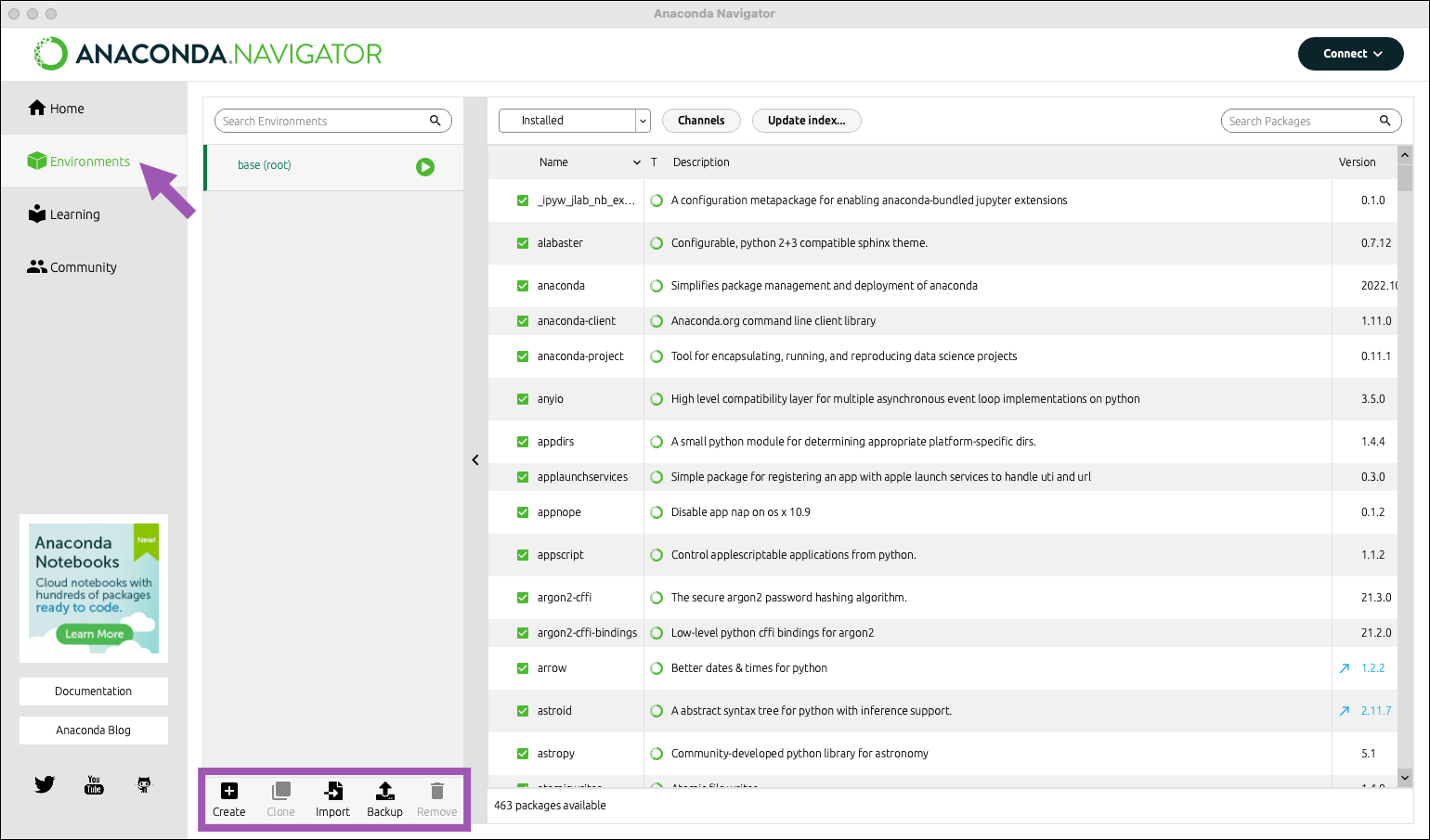 + +2. At the bottom of the environments list, click *Create*. + +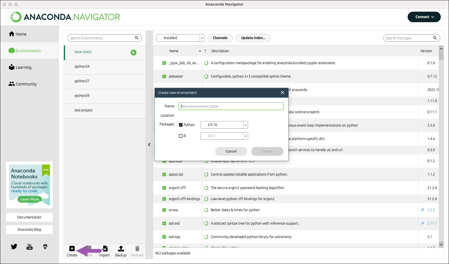 + +3. Select the python checkbox. + +4. Select versions of python. At the time of making this tutorial the latest version of Python is 3.xx.x. We will go ahead and use that one. + +5. Choose an appropriate name for your project. We will be creating an environment for the Spyder IDE so we'll call it "spyder-dev". + +6. Click *Create*. + +For more information see [Anaconda Environments](https://docs.anaconda.com/working-with-conda/environments/) and [Managing environment](https://docs.anaconda.com/navigator/tutorials/manage-environments/). + +## Package Management +Now that we have a clean environment configured, let us install some library we will be using for this class. + +1. Navigate to the environment page and select the environment we just created in the previous section. + +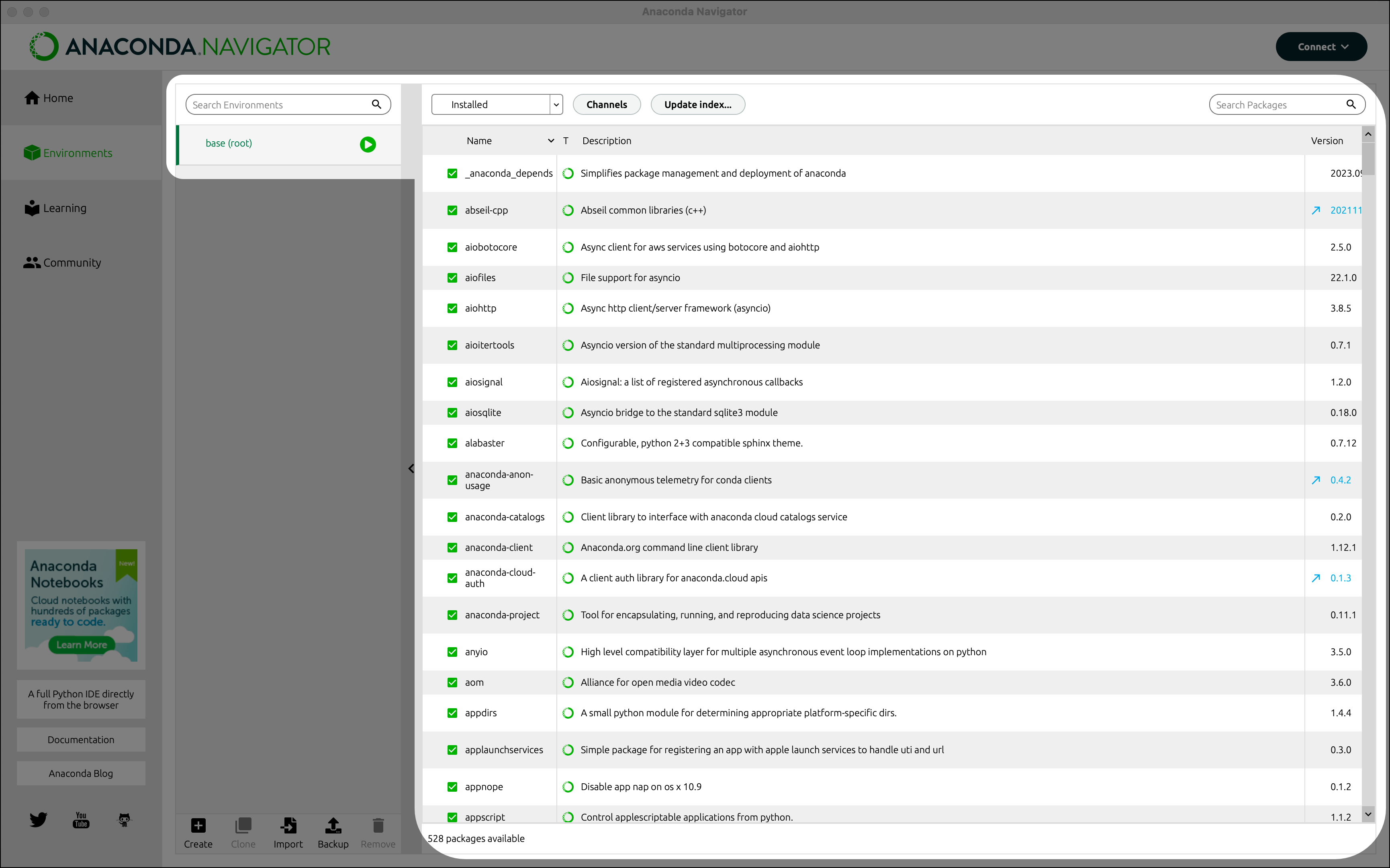 + +2. Use the search bar in the top right corner to search for the following packages: + +| Library | Usage | +| ---------- | --------------------------------- | +| numpy | Numerical computation | +| scipy | Scientific and techical computing | +| pandas | Data manipulation and analysis | +| matplotlib | Plots and visualizations | +| sympy | Symbolic mathematics | +*Note: The libraries list may change throughout the development of this course* + +3. Check the boxes to install the selected packages to the current environment. + +## Installing Applications +From the *Home* page you can install applications, to the current environment we created in the Environment section above. In this section we will install Spyder IDE, but the process is exactly the same for other applications. + +1. Go to the *Home* page. + +2. Select the desired environment. In our case, we select Spyder-dev. + +3. From the Home page find the Spyder IDE tile. Click the *Install* button to start the download. + +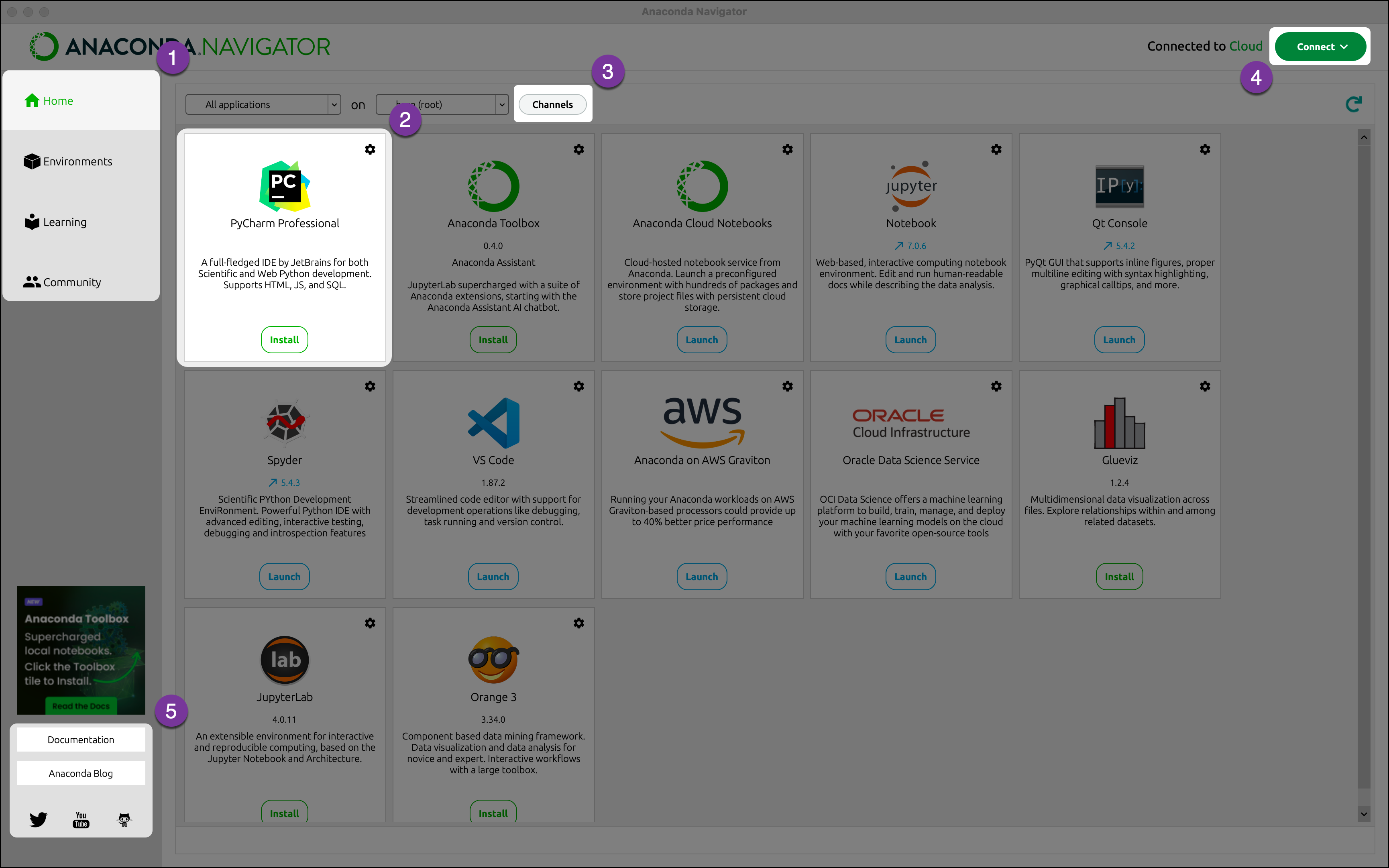 + +4. Once the download is complete, press *Launch* to start the applications.
\ No newline at end of file diff --git a/tutorials/module_1/1_04_spyder_getting_started.md b/tutorials/module_1/1_04_spyder_getting_started.md new file mode 100644 index 0000000..ba055d7 --- /dev/null +++ b/tutorials/module_1/1_04_spyder_getting_started.md @@ -0,0 +1,41 @@ +# Getting started with Spyder + +In this tutorial we will cover the basics of using the Spyder IDE (Interactive Development Environment). If you've ever worked with MATLAB before, then this will feel familiar. Spyder is a program that allows you to write, run and de-bug code. + +## Launching Spyder +Using Anaconda we will select the environment we created earlier *spyder-dev* and then we can launch spyder from the Home page. + +## Spyder Interface + +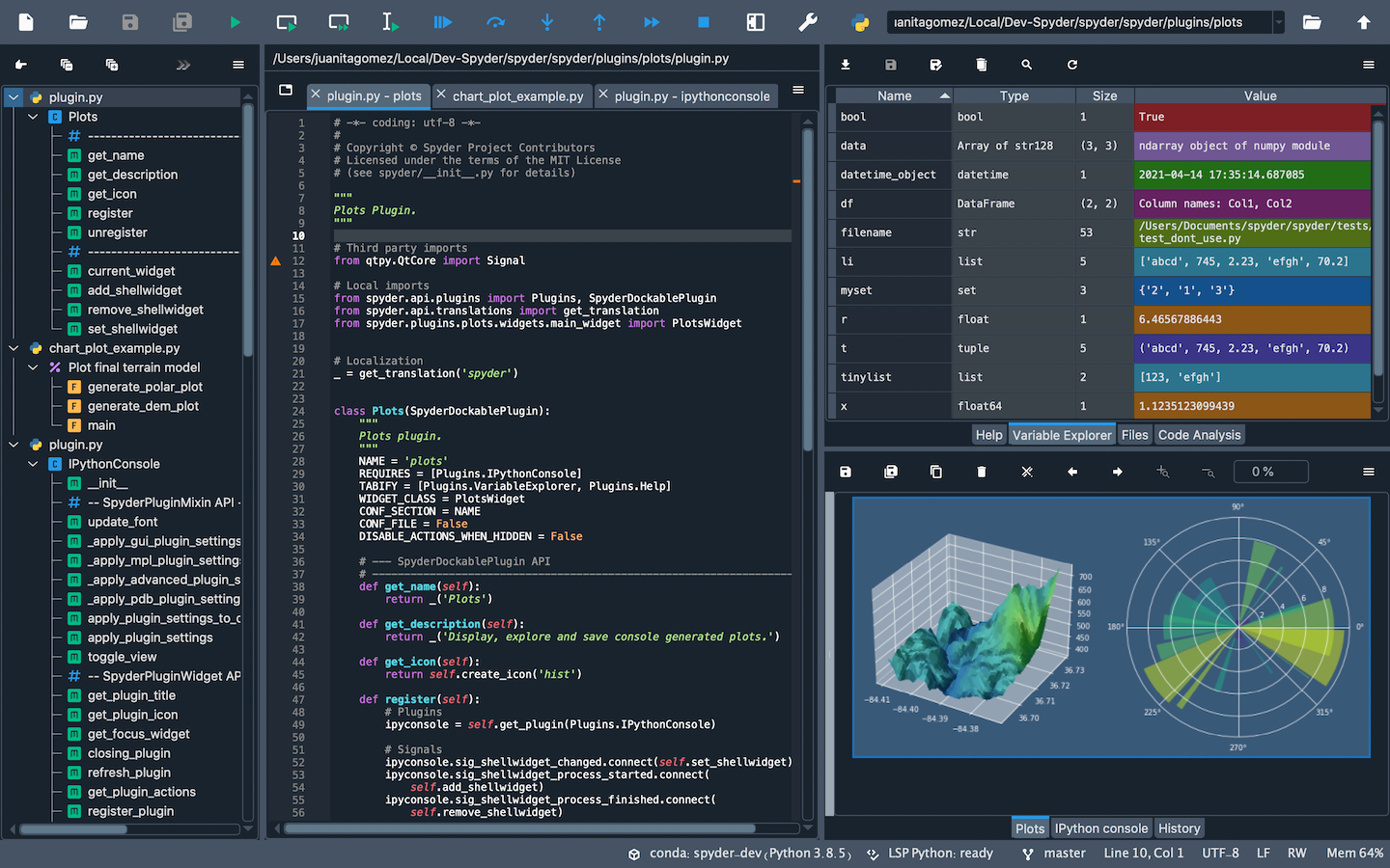 + +Once you open up Spyder in it's default configuration, you'll see three sections; the editor IPython Console, Help viewer. You can customize the interface to suit your prefference and needs some of which include, rearrange, undock, hide panes. Feel free to set up Spyder as you like. + +### Editor +This pane is used to write your scripts. The + +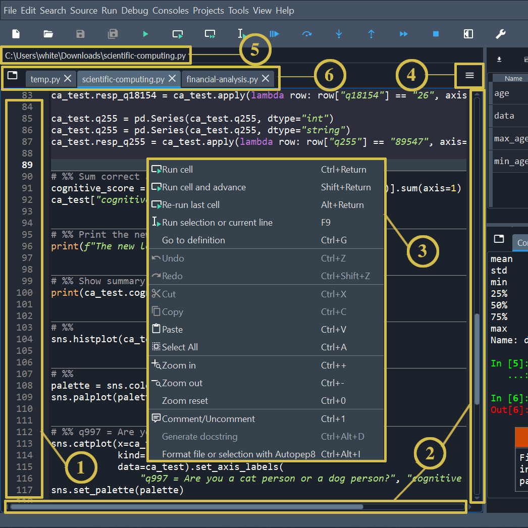 + +1. The left sidebar shows line numbers and displays any code analysis warnings that exist in the current file. Clicking a line number selects the text on that line, and clicking to the right of it sets a [breakpoint](https://docs.spyder-ide.org/5/panes/debugging.html#debugging-breakpoints). +2. The scrollbars allow vertical and horizontal navigation in a file. +3. The context (right-click) menu displays actions relevant to whatever was clicked. +4. The options menu (“Hamburger” icon at top right) includes useful settings and actions relevant to the Editor. +5. The location bar at the top of the Editor pane shows the full path of the current file. +6. The tab bar displays the names of all opened files. It also has a Browse tabs button (at left) to show every open tab and switch between them—which comes in handy if many are open. + +### IPython Console +This pane allows you to interactively run functions, do math computations, assign and modify variables. + +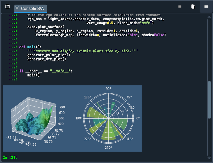 + +- Automatic code completion +- Real-time function calltips +- Full GUI integration with the enhanced Spyder [Debugger](https://docs.spyder-ide.org/5/panes/debugging.html). +- The [Variable Explorer](https://docs.spyder-ide.org/5/panes/variableexplorer.html), with GUI-based editors for many built-in and third-party Python objects. +- Display of Matplotlib graphics in Spyder’s [Plots](https://docs.spyder-ide.org/5/panes/plots.html) pane, if the Inline backend is selected under Preferences ‣ IPython console ‣ Graphics ‣ Graphics backend, and inline in the console if Mute inline plotting is unchecked under the Plots pane’s options menu. + +### Variable Explorer +This pane shows all the defined variables (objects) stored. This can be used to identify the data type of variables, the size and inspect larger arrays. Double clicking the value cell opens up a window which allowing you to inspect the data in a spreadsheet like view. + +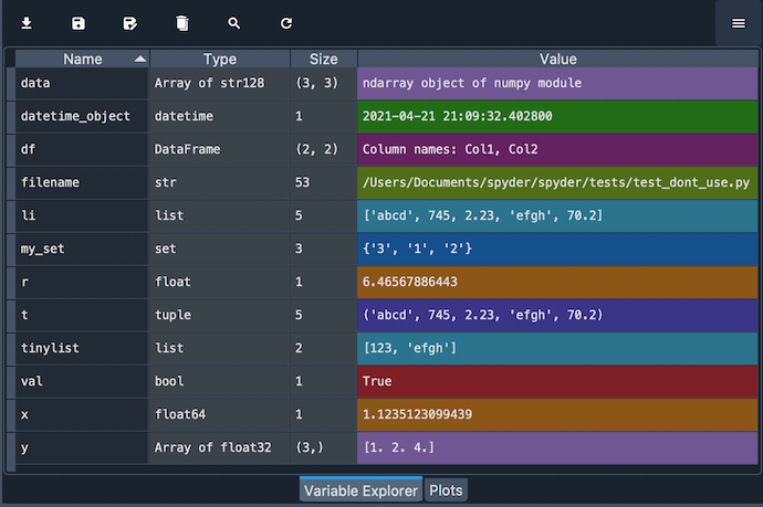 + diff --git a/tutorials/module_1/1_05_basics_of_python.md b/tutorials/module_1/1_05_basics_of_python.md new file mode 100644 index 0000000..5cc9aee --- /dev/null +++ b/tutorials/module_1/1_05_basics_of_python.md @@ -0,0 +1,160 @@ +# Basics of Python + +This page contains important fundamental concepts used in Python such as syntax, operators, order or precedence and more. + +[Syntax](1_05_basics_of_python#Syntax) +[Operators](1_05_basics_of_python#Operators) +[Order of operation](1_05_basics_of_python#Order%20of%20Operation) +[Data types](1_05_basics_of_python#data%20types) +[Variables](1_05_basics_of_python#Variables) + +--- +## Syntax +### Indentations and blocks +In python *indentations* or the space at the start of each line, signifies a block of code. This becomes important when we start working with function and loops. We will talk more about this in the controls structures tutorial. +### Comments +Comments can be added to your code using the hash operator (#). Any text behind the comment operator till the end of the line will be rendered as a comment. +If you have an entire block of text or code that needs to be commented out, the triple quotation marks (""") can be used. Once used all the code after it will be considered a comment until the comment is ended with the triple quotation marks.f + +--- +## Operators +In python, operators are special symbols or keywords that perform operations on values or variables. This section covers some of the most common operator that you will see in this course. +### Arithmetic operators +| Operator | Name | +| --- | --- | +| + | Addition | +| - | Subtraction | +| * | Multiplication | +| / | Division | +| % | Modulus | +| ** | Exponentiation | +| // | Floor division | + + +### Comparison operators +Used in conditional statements such as `if` statements or `while` loops. Note that in the computer world a double equal sign (`==`) means *is equal to*, where as the single equal sign assigns the variable or defines the variable to be something. + +| Operator | Name | +| --- | --- | +| == | Equal | +| != | Not equal | +| > | Greater than | +| < | Less than | +| >= | Greater than or equal to | +| <= | Less than or equal to | + +### Logical operators +| Operator | Descrription | +| --- | --- | +| and | Returns True if both statemetns are true | +| or | Returns True if one of the statements is true | +| not | Reerse the result, returns False if the result is true | + +### Identity operators +| Operator | Description | +| --- | --- | +| is | Returns True if both variables are the same object | +| is not | Returns True if both variables are not the same object | + +--- +## Order of Operation +Similarly to the order or precedence in mathematics, different computer languages have their own set of rules. Here is a comprehensive table of the order of operation that python follows. + +| Operator | Description | +| ------------------------------------------------------- | ----------------------------------------------------- | +| `()` | Parentheses | +| `**` | Exponentiation | +| `+x` `-x` `~x` | Unary plus, unary minus, and bitwise NOT | +| `*` `/` `//` `%` | Multiplication, Division, floor division, and modulus | +| `+` `-` | Addition and subtraction | +| `<<` `>>` | Bitwise left and right shifts | +| & | Bitwise AND | +| ^ | Bitwise XOR | +| \| | Bitwise OR | +| `==` `!=` `>` `>=` `<` `<=` `is` `is not` `in` `not in` | Comparision, identity and membership operators | +| `not` | logical NOT | +| `and` | AND | +| `or` | OR | + +--- +## Data types +Data types are different ways a computer stores data. Other data types use fewer bits than others allowing you to better utilize your computer memory. This is important for engineers because +The most common data types that an engineer encounters in python are numeric types. +- `int` - integer +- `float` - a decimal number +- `complex` - imaginary number + +The comprehensive table below show all built-in data types available in python. + +| Category | Data Type | +| -------- | ---------------------------- | +| Text | int, float, complex | +| Sequance | list, tuple, range | +| Mapping | dict | +| Set | set, frozenset | +| Boolean | bytes, bytearray, memoryview | +| Binary | bytes, bytearray, memoryview | +| None | NoneType | + +--- +## Variables + +A **variable** in Python is a name that stores a value, allowing you to use and manipulate data efficiently. + +#### Declaring and Assigning Variables + +It is common in low-level computer languages to declare the datatype if the variable. In python, the datatype is set whilst you assign it. We assign values to variables using a single `=`. + +```python +x = 10 # Integer +y = 3.14 # Float +name = "Joe" # String +is_valid = True # Boolean +``` + +You can assign multiple variables at once: + +```python +a, b, c = 1, 2, 3 +``` + +Similarly we can assign the same value to multiple variables: + +```python +x = y = z = 100 +``` +##### Rules + +- Must start with a letter or `_` +- Cannot start with a number +- Can only contain letters, numbers, and `_` +- Case-sensitive (`Name` and `name` are different) + +#### Updating Variables + +You can change a variable’s value at any time. + +```python +x = 5 +x = x + 10 # Now x is 15 +``` + +Or shorthand: + +```python +x += 10 # Same as x = x + 10 +``` + +#### Variable Types & Type Checking + +Use `type()` to check a variable’s type. + +```python +x = 10 +print(type(x)) # Output: <class 'int'> + +y = "Hello" +print(type(y)) # Output: <class 'str'> +``` + + diff --git a/tutorials/module_1/1_06_array.md b/tutorials/module_1/1_06_array.md new file mode 100644 index 0000000..c8f2452 --- /dev/null +++ b/tutorials/module_1/1_06_array.md @@ -0,0 +1,169 @@ +# Arrays + +In computer programming, an array is a structure for storing and retrieving data. We often talk about an array as if it were a grid in space, with each cell storing one element of the data. For instance, if each element of the data were a number, we might visualize a “one-dimensional” array like a list: + +| 1 | 5 | 2 | 0 | +| --- | --- | --- | --- | + +A two-dimensional array would be like a table: + +| 1 | 5 | 2 | 0 | +| --- | --- | --- | --- | +| 8 | 3 | 6 | 1 | +| 1 | 7 | 2 | 9 | + +A three-dimensional array would be like a set of tables, perhaps stacked as though they were printed on separate pages. If we visualize the position of each element as a position in space. Then we can represent the value of the element as a property. In other words, if we were to analyze the stress concentration of an aluminum block, the property would be stress. + +- From [Numpy documentation](https://numpy.org/doc/2.2/user/absolute_beginners.html) + + +If the load on this block changes over time, then we may want to add a 4th dimension i.e. additional sets of 3-D arrays for each time increment. As you can see - the more dimensions we add, the more complicated of a problem we have to solve. It is possible to increase the number of dimensions to the n-th order. This course we will not be going beyond dimensional analysis. + +--- +# Numpy - the python's array library + +In this tutorial we will be introducing arrays and we will be using the numpy library. Arrays, lists, vectors, matrices, sets - You might've heard of them before, they all store data. In programming, an array is a variable that can hold more than one value at a time. We will be using the Numpy python library to create arrays. Since we already have installed Numpy previously, we can start using the package. + +Before importing our first package, let's as ourselves *what is a package?* A package can be thought of as pre-written python code that we can re-use. This means the for every script that we write in python we need to tell it to use a certain package. We call this importing a package. + +## Importing Numpy +When using packages in python, we need to let it know what package we will be using. This is called importing. To import numpy we need to declare it a the start of a script as follows: +```python +import numpy as np +``` +- `import` - calls for a library to use, in our case it is Numpy. +- `as` - gives the library an alias in your script. It's common convention in Python programming to make the code shorter and more readable. We will be using *np* as it's a standard using in many projects. + +--- +# Creating arrays +Now that we have imported the library we can create a one dimensional array or *vector* with three elements. +```python +x = np.array([1,2,3]) +``` + + +To create a *matrix* we can nest the arrays to create a two dimensional array. This is done as follows. + +```python +matrix = np.array([[1,2,3], + [4,5,6], + [7,8,9]]) +``` + +*Note: for every array we nest, we get a new dimension in our data structure.* + +## Numpy array creation functions +Numpy comes with some built-in function that we can use to create arrays quickly. Here are a couple of functions that are commonly used in python. +### np.arange +The `np.arange()` function returns an array with evenly spaced values within a specified range. It is similar to the built-in `range()` function in Python but returns a Numpy array instead of a list. The parameters for this function are the start value (inclusive), the stop value (exclusive), and the step size. If the step size is not provided, it defaults to 1. + +```python +>>> np.arange(4) +array([0. , 1., 2., 3. ]) +``` + +In this example, `np.arange(4)` generates an array starting from 0 and ending before 4, with a step size of 1. + +### np.linspace +The `np.linspace()` function returns an array of evenly spaced values over a specified range. Unlike `np.arange()`, which uses a step size to define the spacing between elements, `np.linspace()` uses the number of values you want to generate and calculates the spacing automatically. It accepts three parameters: the start value, the stop value, and the number of samples. + +```python +>>> np.linspace(1., 4., 6) +array([1. , 1.6, 2.2, 2.8, 3.4, 4. ]) +``` + +In this example, `np.linspace(1., 4., 6)` generates 6 evenly spaced values between 1. and 4., including both endpoints. + +Try this and see what happens: + +```python +x = np.linspace(0,100,101) +y = np.sin(x) +``` + +### Other useful functions +- `np.zeros()` +- `np.ones()` +- `np.eye()` + +## Working with Arrays +Now that we have been introduced to some ways to create arrays using the Numpy functions let's start using them. +### Indexing +Indexing in Python allows you to access specific elements within an array based on their position. This means you can directly retrieve and manipulate individual items as needed. + +Python uses **zero-based indexing**, meaning the first element is at position **0** rather than **1**. This approach is common in many programming languages. For example, in a list with five elements, the first element is at index `0`, followed by elements at indices `1`, `2`, `3`, and `4`. + +Here's an example of data from a rocket test stand where thrust was recorded as a function of time. + +```python +thrust_lbf = np.array(0.603355, 2.019083, 2.808092, 4.054973, 1.136618, 0.943668) + +>>> thrust_lbs[3] +``` + +Due to the nature of zero-based indexing. If we want to call the value `4.054973` that will be the 3rd index. +### Operations on arrays +- Arithmetic operations (`+`, `-`, `*`, `/`, `**`) +- `np.add()`, `np.subtract()`, `np.multiply()`, `np.divide()` +- `np.dot()` for dot product +- `np.matmul()` for matrix multiplication +- `np.linalg.inv()`, `np.linalg.det()` for linear algebra +#### Statistics +- `np.mean()`, `np.median()`, `np.std()`, `np.var()` +- `np.min()`, `np.max()`, `np.argmin()`, `np.argmax()` +- Summation along axes: `np.sum(arr, axis=0)` +#### Combining arrays +- Concatenation: `np.concatenate((arr1, arr2), axis=0)` +- Stacking: `np.vstack()`, `np.hstack()` +- Splitting: `np.split()` + +# Exercise +Let's solve a statics problem given the following problem + +A simply supported bridge of length L=20L = 20L=20 m is subjected to three point loads: + +- $P1=10P_1 = 10P1=10 kN$ at $x=5x = 5x=5 m$ +- $P2=15P_2 = 15P2=15 kN$ at $x=10x = 10x=10 m$ +- $P3=20P_3 = 20P3=20 kN$ at $x=15x = 15x=15 m$ + +The bridge is supported by two reaction forces at points AAA (left support) and BBB (right support). We assume the bridge is in static equilibrium, meaning the sum of forces and sum of moments about any point must be zero. + +#### Equilibrium Equations: + +1. **Sum of Forces in the Vertical Direction**: + $RA+RB−P1−P2−P3=0R_A + R_B - P_1 - P_2 - P_3 = 0RA+RB−P1−P2−P3=0$ +2. **Sum of Moments About Point A**: + $5P1+10P2+15P3−20RB=05 P_1 + 10 P_2 + 15 P_3 - 20 R_B = 05P1+10P2+15P3−20RB=0$ +3. **Sum of Moments About Point B**: + $20RA−15P3−10P2−5P1=020 R_A - 15 P_3 - 10 P_2 - 5 P_1 = 020RA−15P3−10P2−5P1=0$ + +#### System of Equations: + +{RA+RB−10−15−20=05(10)+10(15)+15(20)−20RB=020RA−5(10)−10(15)−15(20)=0\begin{cases} R_A + R_B - 10 - 15 - 20 = 0 \\ 5(10) + 10(15) + 15(20) - 20 R_B = 0 \\ 20 R_A - 5(10) - 10(15) - 15(20) = 0 \end{cases}⎩ + + +## Solution +```python +import numpy as np + +# Define the coefficient matrix A +A = np.array([ + [1, 1], + [0, -20], + [20, 0] +]) + +# Define the right-hand side vector b +b = np.array([ + 45, + 5*10 + 10*15 + 15*20, + 5*10 + 10*15 + 15*20 +]) + +# Solve the system of equations Ax = b +x = np.linalg.lstsq(A, b, rcond=None)[0] # Using least squares to handle potential overdetermination + +# Display the results +print(f"Reaction force at A (R_A): {x[0]:.2f} kN") +print(f"Reaction force at B (R_B): {x[1]:.2f} kN") +```
\ No newline at end of file diff --git a/tutorials/module_1/1_07_control_structures.md b/tutorials/module_1/1_07_control_structures.md new file mode 100644 index 0000000..15e97eb --- /dev/null +++ b/tutorials/module_1/1_07_control_structures.md @@ -0,0 +1,127 @@ +# Control Structures +Control structures allow us to control the flow of execution in a Python program. The two main types are **conditional statements (`if` statements)** and **loops (`for` and `while` loops)**. + +## Conditional Statements + +Conditional statements allow a program to execute different blocks of code depending on whether a given condition is `True` or `False`. These conditions are typically comparisons, such as checking if one number is greater than another. + +### The `if` Statement + +The simplest form of a conditional statement is the `if` statement. If the condition evaluates to `True`, the indented block of code runs. Otherwise, the program moves on without executing the statement. + +For example, consider a situation where we need to determine if a person is an adult based on their age. If the age is 18 or greater, we print a message saying they are an adult. + +### The `if-else` Statement + +Sometimes, we need to specify what should happen if the condition is `False`. The `else` clause allows us to handle this case. Instead of just skipping over the block, the program can execute an alternative action. + +For instance, if a person is younger than 18, they are considered a minor. If the condition of being an adult is not met, the program will print a message indicating that the person is a minor. + +### The `if-elif-else` Statement + +When dealing with multiple conditions, the `if-elif-else` structure is useful. The program evaluates conditions in order, executing the first one that is `True`. If none of the conditions are met, the `else` block runs. + +For example, in a grading system, different score ranges correspond to different letter grades. If a student's score is 90 or higher, they receive an "A". If it's between 80 and 89, they get a "B", and so on. If none of the conditions match, they receive an "F". + +### Nested `if` Statements + +Sometimes, we need to check conditions within other conditions. This is known as **nesting**. For example, if we first determine that a person is an adult, we can then check if they are a student. Based on that information, we print different messages. + + +```python +# Getting user input for the student's score +score = int(input("Enter the student's score (0-100): ")) + +if 0 <= score <= 100: + if score >= 90: + grade = "A" + elif score >= 80: + grade = "B" + elif score >= 70: + grade = "C" + elif score >= 60: + grade = "D" + else: + grade = "F" # Score below 60 is a failing grade + + + if grade == "F": + print("The student has failed.") + retake_eligible = input("Is the student eligible for a retest? (yes/no): ").strip().lower() + + if retake_eligible == "yes": + print("The student is eligible for a retest.") + else: + print("The student has failed the course and must retake it next semester.") + + +``` + +--- + +## Loops in Python + +Loops allow a program to execute a block of code multiple times. This is especially useful for tasks such as processing lists of data, performing repetitive calculations, or automating tasks. + +### The `for` Loop + +A `for` loop iterates over a sequence, such as a list, tuple, string, or a range of numbers. Each iteration assigns the next value in the sequence to a loop variable, which can then be used inside the loop. + +For instance, if we have a list of fruits and want to print each fruit's name, a `for` loop can iterate over the list and display each item. + +Another useful feature of `for` loops is the `range()` function, which generates a sequence of numbers. This is commonly used when we need to repeat an action a specific number of times. For example, iterating from 0 to 4 allows us to print a message five times. + +Additionally, the `enumerate()` function can be used to loop through a list while keeping track of the index of each item. This is useful when both the position and the value in a sequence are needed. + +```python +fruits = ["apple", "banana", "cherry"] +for x in fruits: + print(x) +``` + +```python +for x in range(6): + print(x) +else: + print("Finally finished!") +``` +### The `while` Loop + +Unlike `for` loops, which iterate over a sequence, `while` loops continue running as long as a specified condition remains `True`. This is useful when the number of iterations is not known in advance. + +For example, a countdown timer can be implemented using a `while` loop. The loop will continue decreasing the count until it reaches zero. + +It's important to be careful with `while` loops to avoid infinite loops, which occur when the condition never becomes `False`. To prevent this, ensure that the condition will eventually change during the execution of the loop. + +A `while` loop can also be used to wait for a certain event to occur. For example, in interactive programs, a `while True` loop can keep running until the user provides a valid input, at which point we break out of the loop. + +```python +i = 1 +while i < 6: + print(i) + i += 1 +``` + +--- + +## Loop Control Statements + +Python provides special statements to control the behavior of loops. These can be used to break out of a loop, skip certain iterations, or simply include a placeholder for future code. + +### The `break` Statement + +The `break` statement is used to exit a loop before it has iterated through all its elements. When the `break` statement is encountered, the loop stops immediately, and the program continues executing the next statement outside the loop. + +For instance, if we are searching for a specific value in a list, we can use a `break` statement to stop the loop as soon as we find the item, instead of continuing unnecessary iterations. + +### The `continue` Statement + +The `continue` statement is used to skip the current iteration and proceed to the next one. Instead of exiting the loop entirely, it simply moves on to the next cycle. + +For example, if we are iterating over numbers and want to skip processing number 2, we can use `continue`. The loop will ignore that iteration and proceed with the next number. + +### The `pass` Statement + +The `pass` statement is a placeholder that does nothing. It is useful when a block of code is syntactically required but no action needs to be performed yet. + +For example, in a loop where a condition has not yet been implemented, using `pass` ensures that the code remains valid while avoiding errors. diff --git a/tutorials/module_1/1_classes_and_objects.md b/tutorials/module_1/1_classes_and_objects.md new file mode 100644 index 0000000..0392483 --- /dev/null +++ b/tutorials/module_1/1_classes_and_objects.md @@ -0,0 +1,8 @@ +# Modular Programming + +Classes and Objects + +## What are they? + + +## Why do we care? diff --git a/tutorials/module_1/1_computational_expense.md b/tutorials/module_1/1_computational_expense.md new file mode 100644 index 0000000..c9631e1 --- /dev/null +++ b/tutorials/module_1/1_computational_expense.md @@ -0,0 +1,2 @@ +# Computational Expense + diff --git a/tutorials/module_1/1_computing_fundamentals.md b/tutorials/module_1/1_computing_fundamentals.md new file mode 100644 index 0000000..1fef338 --- /dev/null +++ b/tutorials/module_1/1_computing_fundamentals.md @@ -0,0 +1,15 @@ +# Computing Fundamentals + +## Using computers as a tool for engineers + +## How do computers work? +Globe analogy: Hardware, Kernel, Shell, Application, Software. + +## Interfaces + +### Text editor for Scripting + + + +### Command window +Command window, terminal, console, command prompt you might've heard of theses terms before. They all essentially mean the same thing. The command window is used to control your system. diff --git a/tutorials/module_1/1_functions.md b/tutorials/module_1/1_functions.md new file mode 100644 index 0000000..8235fe3 --- /dev/null +++ b/tutorials/module_1/1_functions.md @@ -0,0 +1,67 @@ +# Functions + +Like a traditional mathematical functions, python functions can take an input, process it, and give an output. In python, the input variables are referred to as *arguments*. Functions are blocks of code that is run every time it's called. This allows us to re-use code. + +Functions are defined by using the <code> def </code> keyword. Reminder: it is important to keep track of indentations as it signifies the end of the function when the indentation returns back to the same level. + +## Defining Functions +### Simple function +A simple function with no input variable can be useful if you need to re-use code multiple times without having to re-write it. + +```python + def function_name(): + print("This is from a function") +``` + +### Defining a function with one input +We can pass variables through to the function to be processed as follows: + +```python + def function(x): + print(x + " is best") +``` + +Note input variables can be of any data type (integer, float, string, etc.). +### Returning values from a function +If we want to calculate a value and pass it back to the script for further use, we can use the `return` keyword. Let's define a linear function that takes two inputs, `x` and `b`, computes the corresponding `y` value, and returns it so it can be used elsewhere in the code. + +```python + def function(x, b): + y = 3*x+b + return y +``` + +For multiple output variables we can add +## Calling functions +Now that we've covered defining functions we want to call the function in order to execute the block inside the function. To do this, we simply re-call the function name as follows. + +```python +function(2,-1) +``` + +Note that when running this code, nothing happens. This is because we haven't told the computer what to do with the output. Hence, if we wish to store the output then we need to use the assign operator `=`. + +```python +output = function(2,-1) + +print(output) +``` + +In case you want to return multiple output variable from a single function we will have... + +## Summary + +```python +def function_name(argument1, argument2, argument3) + output1 = argument1 * argument2 - argument3 + output2 = argument2 + argument3 + return output1, output2 + +[solution1, solution2] = function_name(1,2,3) +``` + + +- `def` - defines a function. All the code that is indented underneath is considered inside the function block. +- `function_name` - this is used to call the function block. +- `argument1` (optional) - input variable. This is data that can be pass to the function. It is possible to have multiple variables separated by a comma. As well as can be omitted if the function should just give you an output such as. +- `return` (optional) - if you wish to return something to your script, the return keyword is used. The keyword can be followed by an output variable or a constant. For multiple output variables, separate them by a comma.
\ No newline at end of file diff --git a/tutorials/module_1/1_fundamentals_of_programming.md b/tutorials/module_1/1_fundamentals_of_programming.md new file mode 100644 index 0000000..617d2c3 --- /dev/null +++ b/tutorials/module_1/1_fundamentals_of_programming.md @@ -0,0 +1,15 @@ +# Fundamentals of programming +## Orientation of common interfaces +In this section we will cover the use and purpose of some common interfaces that you'll be using in this course. + +### Command window, terminal, console, command prompt. +This is a text based interface that allows the users to interact with the computer. It is used to execute commands, run scripts or programs. + + +### Text Editor / Script +Your text editor is the program used to write a script which can be re-run every time you call it from the command window. This can be a built-in text editor such as Spyder and MATLAB provide or an external on such a notepad++. + + + + Globe analogy: Hardware, Kernel, shell, Application software. + - Scripting
\ No newline at end of file diff --git a/tutorials/module_1/1_open_source_software.md b/tutorials/module_1/1_open_source_software.md new file mode 100644 index 0000000..924878b --- /dev/null +++ b/tutorials/module_1/1_open_source_software.md @@ -0,0 +1,41 @@ +# Open Source Software + +Open-source software (OSS) is a type of software that allows users to access, modify, and distribute its source code freely. It is built on principles of collaboration, transparency, and community-driven development. + +### Key Principles of Open Source Software + +- **Free Distribution:** Anyone can download and use the software without cost. +- **Access to Source Code:** Users can view and modify the code to suit their needs. +- **Community Collaboration:** Developers from around the world contribute to improvements and security fixes. + +### Benefits of Open Source Software + +- **Cost-effectiveness:** Open-source software is free to use, making it accessible to individuals and organizations. +- **Transparency and Security:** Open code allows for peer review, reducing security vulnerabilities. +- **Community Support:** Global developer communities provide assistance, troubleshooting, and improvements. +- **Customization and Flexibility:** Users can modify software to fit their specific requirements. + +### Challenges of Open Source Software + +- **Usability Issues:** Some open-source software may have a steeper learning curve. +- **Compatibility Problems:** Integration with proprietary systems may require additional effort. +- **Support and Documentation:** The quality of documentation and support varies. +- **Sustainability:** Open-source projects often rely on volunteers, which can lead to inconsistent updates. + +### Popular Open Source Projects + +- **Operating Systems:** Linux, Ubuntu +- **Web Browsers:** Mozilla Firefox +- **Programming Languages:** Python, JavaScript +- **Office Suites:** LibreOffice +- **Multimedia Tools:** Audacity, Blender +- **Software Development:** Git, GitHub, Apache + +### How to Contribute to Open Source + +- **Finding Projects:** Platforms like GitHub, GitLab, and SourceForge host many open-source projects. +- **Understanding Licensing:** Common licenses include GPL, MIT, and Apache. +- **Ways to Contribute:** Developers can contribute code, test software, write documentation, translate, or help with design. +- **Best Practices for Contributions:** Using version control (Git), writing clean code, and following community guidelines are essential for successful collaboration. + +## Licensing |