
diff options
| author | Christian Kolset <christian.kolset@gmail.com> | 2025-09-10 14:21:30 -0600 |
|---|---|---|
| committer | Christian Kolset <christian.kolset@gmail.com> | 2025-09-10 14:21:30 -0600 |
| commit | e6244e2c4f1c8b241f822cdf25b36fb3fa6cc33e (patch) | |
| tree | f47373c6e0d3d1d92feb14f91c04b66603ab5068 /tutorials/module_3 | |
| parent | 9842533cf12a9878535b3539291a527c1511b45c (diff) | |
Added newton-raphson material and inclused recursive vs iterative approaches
Diffstat (limited to 'tutorials/module_3')
| -rw-r--r-- | tutorials/module_3/2_roots_optimization.md | 68 |
1 files changed, 55 insertions, 13 deletions
diff --git a/tutorials/module_3/2_roots_optimization.md b/tutorials/module_3/2_roots_optimization.md index 2c94f92..3d126e0 100644 --- a/tutorials/module_3/2_roots_optimization.md +++ b/tutorials/module_3/2_roots_optimization.md @@ -54,12 +54,21 @@ This exact same concept can be applied to finding roots of functions. Instead of > The **Intermediate Value Theorem** says that if f(x) is a continuous function between a and b, and sign(f(a))≠sign(f(b)), then there must be a c, such that a<c<b and f(c)=0. Let's consider a continuous function $f(x)$ with an unknown root $x_r$ . Using the intermediate value theorem we can bracket a root with the points $x_{lower}$ and $x_{upper}$ such that $f(x_{lower})$ and $f(x_{upper})$ have opposite signs. This idea is visualized in the graph below. - -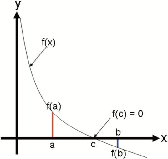 - +<img + style="display: block; + margin-left: auto; + margin-right: auto; + width: 50%;" + src="https://pythonnumericalmethods.studentorg.berkeley.edu/_images/19.03.01-Intermediate-value-theorem.png" + alt="Intermediate Value Theorem"> Once we bisect the interval and found we set the new predicted root to be in the middle. We can then compare the two sections and see if there is a sign change between the bounds. Once the section with the sign change has been identified, we can repeat this process until we near the root. - -![[bisection.png|500]] +<img + style="display: block; + margin-left: auto; + margin-right: auto; + width: 50%;" + src="bisection.png" + alt="Bisection"> As you the figure shows, the predicted root $x_r$ get's closer to the actual root each iteration. In theory this is an infinite process that can keep on going. In practice, computer precision may cause error in the result. A work-around to these problems is setting a tolerance for the accuracy. As engineers it is our duty to determine what the allowable deviation is. So let's take a look at how we can write this in python. @@ -128,23 +137,53 @@ plt.legend() plt.show() ``` # Open Methods -So far we looked at methods that require us to bracket a root before finding it. However, let's think outside of the box and ask ourselves if we can find a root with only 1 guess. Can we improve the our guess by if we have some knowledge of the function itself? +So far we looked at methods that require us to bracket a root before finding it. However, let's think outside of the box and ask ourselves if we can find a root with only 1 guess. Can we improve the our guess by if we have some knowledge of the function itself? The answer - derivatives. ## Newton-Raphson -Possibly the most used root finding method implemented in algorithms is the Newton-Raphson method. Unlike the bracketing methods, we use one guess and the slope of the function to find our next guess. We can represent this graphically below. - -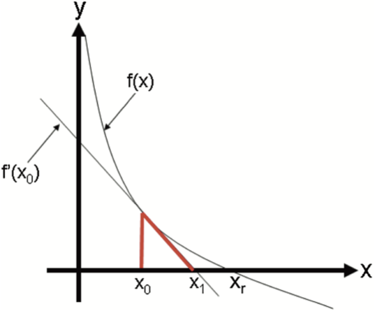 - - +Possibly the most used root finding method implemented in algorithms is the Newton-Raphson method. By using the initial guess we can draw a tangent line at this point on the curve. Where the tangent intercepts the x-axis is usually an improved estimate of the root. It can be more intuitive to see this represented graphically. <img style="display: block; margin-left: auto; margin-right: auto; - width: 60%;" + width: 50%;" src="https://pythonnumericalmethods.studentorg.berkeley.edu/_images/19.04.01-Newton-step.png" alt="Newton-Raphson illustration"> +Given the function $f(x)$ we make our first guess at $x_0$. Using our knowledge of the function at that point we can calculate the derivative to obtain the tangent. Using the equation of the tangent we can re-arrange it to solve for $x$ when $f(x)=0$ giving us our first improved guess $x_1$. -If we start with a single +As seen in the figure above. The derivative of the function is equal to the slope. +$$ +f'(x_0) = \frac{f(x_0)-0}{x_0-x_1} +$$ +Re-arranging for our new guess we get: +$$ +x_{1} = x_0 - \frac{f(x_0)}{f'(x_0)} +$$ +Since $x_0$ is our current guess and $x_0$ is our next guess, we can write these symbolically as $x_i$ and $x_{i+1}$ respectively. This gives us the *Newton-Raphson formula*. +$$ +\boxed{x_{i+1} = x_i - \frac{f(x_i)}{f'(x_i)}} +$$ +### Assignment 2 +Write a python function called *newtonraphson* which as the following input parameters + - `f` - function + - `df` - first derivative of the function + - `x0` - initial guess + - `tol` - the tolerance of error + That finds the root of the function $f(x)=e^{\left(x-6.471\right)}\cdot1.257-0.2$ and using an initial guess of 8. + +```python +def newtonraphson(f, df, x0, tol): + # Output of this function is the estimated root of f + # using the Newton-Raphson method + + if abs(f(x0)) < tol: + return x0 + else: + return newtonraphson(f,df,x0) + +f = lambda x:x**2-1.5 +f_prime = labmda x:2*x + +``` ## Modified Secant This method uses the finite derivative to guess where the root lies. We can then iterate this guessing process until we're within tolerance. @@ -163,6 +202,9 @@ x_{x+1} = x_i - \frac{f(x_i)\delta_x}{f(x_i+\delta x)-f(x_i)} $$ +## Issues with open methods +Diverging guesses + # Pipe Friction Example Numerical methods for Engineers 7th Edition Case study 8.4.
\ No newline at end of file |