1
2
3
4
5
6
7
8
9
10
11
12
13
14
15
16
17
18
19
20
21
22
23
24
25
26
27
28
29
30
31
32
33
34
35
36
37
38
39
40
41
42
43
44
45
46
47
48
49
50
51
52
53
54
55
56
57
58
59
60
61
62
63
64
65
66
67
68
69
70
71
72
73
74
75
76
77
78
79
80
81
82
83
84
85
86
87
88
89
90
91
92
93
94
95
96
97
98
99
100
101
102
103
104
105
106
107
108
109
110
111
112
113
114
115
116
117
118
119
120
121
122
123
124
125
126
127
128
129
130
131
132
133
134
135
136
137
138
139
140
141
142
143
144
145
|
# Root Finding Methods
By now you've learned the quadratic formula to find the roots of a second degree polynomial.
$$
x=\frac{-b \pm \sqrt{b^2-4ac}}{2a}
$$
This works nicely if we're given the function $f(x)$. However, how would you solve for $x$ if you were given experimental data? In this section we will cover bracketing and open methods to find roots of a function.
Let us take a step back and think *algorithmically*. To find a root numerically, we can implement a search algorithm. Let's consider a small phone book - a database of names and numbers sorted alphabetically by last name. Our goal is to find the phone number of James Watt (our root). We could make an algorithm that starts at the the first page, checks to see if the current name equals our target (Watt), if it doesn't, check the next entry. This is method is called *incremental search*. As you may see, this can take very long if the database is large.
> [!NOTE] Example Phonebook Database Entries
> **A** – Archimedes
> **B** – Bernoulli
> **C** – Curie
> **D** – Darwin
> **E** – Einstein
> **F** – Feynman
> **G** – Galileo
> **H** – Hubble
> **I** – Ibn Sina
> **J** – Joule
> **K** – Kelvin
> **L** – Leonardo
> **M** – Maxwell
> **N** – Newton
> **O** – Oppenheimer
> **P** – Pascal
> **Q** – Quetelet
> **R** – Röntgen
> **S** – Schrödinger
> **U** – Urey
> **V** – Volta
> **W** – Watt
> **X** – Xenophon
> **Y** – Yukawa
> **Z** – Zuse
Another approach may be to index the book and jump straight to the 'W' names however this requires two steps.
When
# Bracketing Method
## Incremental Search
Incremental search
## Bisection
This method start by sectioning the database into two halves. We can do this with a phone book by simply opening it in the middle of the book. In our data set, we have find the middle entry to be 'M - Maxwell'. Based on the premises that all names are sorted alphabetically we can conclude that we will find our target in the second half, essentially eliminating the first half. Doing this a second time gives us our new midpoint 'S – Schrödinger' and a third time get us to our target 'W - Watt'. In only 3 iterations we have reached out target goal. This is a huge improvement from the Incremental search (22 iterations) versus our new 3 iterations.
This exact same concept can be applied to finding roots of functions. Instead of searching for strings we are searching for floats. For computers this is a lot easier to do. Take a moment to think about how you would write psuedo-code to program this.
> The **Intermediate Value Theorem** says that if f(x) is a continuous function between a and b, and sign(f(a))≠sign(f(b)), then there must be a c, such that a<c<b and f(c)=0.
Let's consider a continuous function $f(x)$ with an unknown root $x_r$ . Using the intermediate value theorem we can bracket a root with the points $x_{lower}$ and $x_{upper}$ such that $f(x_{lower})$ and $f(x_{upper})$ have opposite signs. This idea is visualized in the graph below.
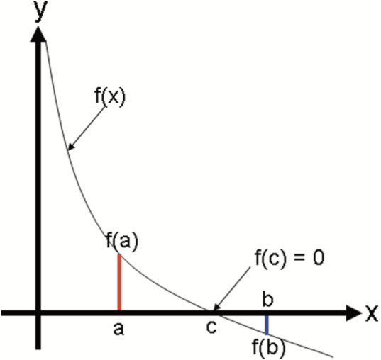
Once we bisect the interval and found we set the new predicted root to be in the middle. We can then compare the two sections and see if there is a sign change between the bounds. Once the section with the sign change has been identified, we can repeat this process until we near the root.
![[Pasted image 20250905120647.png|500]]
As you the figure shows, the predicted root $x_r$ get's closer to the actual root each iteration. In theory this is an infinite process that can keep on going. In practice, computer precision may cause error in the result. A work-around to these problems is setting a tolerance for the accuracy. As engineers it is our duty to determine what the allowable deviation is.
So let's take a look at how we can write this in python.
```python
import numpy as np
def my_bisection(f, x_l, x_u, tol):
# approximates a root, R, of f bounded
# by a and b to within tolerance
# | f(m) | < tol with m the midpoint
# between a and b Recursive implementation
# check if a and b bound a root
if np.sign(f(x_l)) == np.sign(f(x_u)):
raise Exception(
"The scalars x_l and x_u do not bound a root")
# get midpoint
x_r = (x_l + x_u)/2
if np.abs(f(x_r)) < tol:
# stopping condition, report m as root
return x_r
elif np.sign(f(x_l)) == np.sign(f(x_r)):
# case where m is an improvement on a.
# Make recursive call with a = m
return my_bisection(f, x_r, x_u, tol)
elif np.sign(f(x_l)) == np.sign(f(x_r)):
# case where m is an improvement on b.
# Make recursive call with b = m
return my_bisection(f, x_l, x_r, tol)
```
### Example
```python
f = lambda x: x**2 - 2
r1 = my_bisection(f, 0, 2, 0.1)
print("r1 =", r1)
r01 = my_bisection(f, 0, 2, 0.01)
print("r01 =", r01)
print("f(r1) =", f(r1))
print("f(r01) =", f(r01))
```
### Assignment 2
Write an algorithm that uses a combination of the bisection and incremental search to find multiple roots in the first 8 minutes of the data set.
```python
import pandas as pd
import matplotlib.pyplot as plt
# Read the CSV file into a DataFrame called data
data = pd.read_csv('your_file.csv')
# Plot all numeric columns
data.plot()
# Add labels and show plot
plt.xlabel("Time (min)")
plt.ylabel("Strain (kPa)")
plt.title("Data with multiple roots")
plt.legend()
plt.show()
```
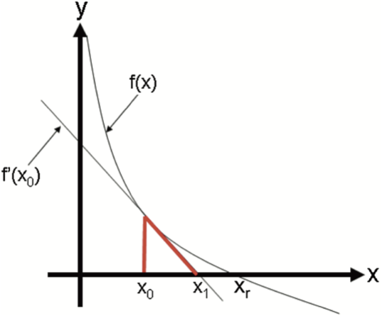
# Open Methods
## Modified Secant
We can do better.
## Newton-Raphson
# Pipe Friction Example
Numerical methods for Engineers 7th Edition Case study 8.4.
|
