
diff options
| author | Christian Kolset <christian.kolset@gmail.com> | 2025-04-24 23:31:17 -0600 |
|---|---|---|
| committer | Christian Kolset <christian.kolset@gmail.com> | 2025-04-24 23:31:17 -0600 |
| commit | c98972ced700b6250915a21af4b76459365743f3 (patch) | |
| tree | 87f62caa9dbe5dbb997f12f7e167ff4ddbc91697 /tutorials/module_1 | |
| parent | 342b88e6002fa1eee9b020864d83ddbd79ef3ad9 (diff) | |
Updated markdown files to look better after converting to latex files.
Diffstat (limited to 'tutorials/module_1')
| -rw-r--r-- | tutorials/module_1/1_excel_to_python.md | 73 | ||||
| -rw-r--r-- | tutorials/module_1/array.md | 2 | ||||
| -rw-r--r-- | tutorials/module_1/intro_to_anaconda.md | 15 | ||||
| -rw-r--r-- | tutorials/module_1/spyder_getting_started.md | 8 |
4 files changed, 85 insertions, 13 deletions
diff --git a/tutorials/module_1/1_excel_to_python.md b/tutorials/module_1/1_excel_to_python.md new file mode 100644 index 0000000..2bf6a0d --- /dev/null +++ b/tutorials/module_1/1_excel_to_python.md @@ -0,0 +1,73 @@ +# Excel to Python + + +- Importing +- Plotting +- Statistical analysis + + + +## **How Excel Translates to Python** + +Here’s how common Excel functionalities map to Python: + +| **Excel Feature** | **Python Equivalent** | +| ----------------------- | -------------------------------------------------------- | +| Formulas (SUM, AVERAGE) | `numpy`, `pandas` (`df.sum()`, `df.mean()`) | +| Sorting & Filtering | `pandas.sort_values()`, `df[df['col'] > value]` | +| Conditional Formatting | `matplotlib` for highlighting | +| Pivot Tables | `pandas.pivot_table()` | +| Charts & Graphs | `matplotlib`, `seaborn`, `plotly` | +| Regression Analysis | `scipy.stats.linregress`, `sklearn.linear_model` | +| Solver/Optimization | `scipy.optimize` | +| VBA Macros | Python scripting with `openpyxl`, `pandas`, or `xlwings` | + +## Statistical functions + +#### SUM +Built-in: +```python +my_array = [1, 2, 3, 4, 5] +total = sum(my_array) +print(total) # Output: 15 +``` +Numpy: +```python +import numpy as np + +my_array = np.array([1, 2, 3, 4, 5]) +total = np.sum(my_array) +print(total) # Output: 15 +``` + +### Average +Built-in: +```python +my_array = [1, 2, 3, 4, 5] +average = sum(my_array) / len(my_array) +print(average) # Output: 3.0 +``` +Numpy: +```python +import numpy as np + +my_array = np.array([1, 2, 3, 4, 5]) +average = np.mean(my_array) +print(average) # Output: 3.0 +``` + + + +## Plotting +We can use the package *matplotlib* to plot our graphs in python. Matplotlib provides data visualization tools for the Scientific Python Ecosystem. You can make very professional looking figures with this tool. + +Here is a section from the matplotlib documentation page that you can run in python. +```python +import matplotlib.pyplot as plt + +fig, ax = plt.subplots() # Create a figure containing a single Axes. +ax.plot([1, 2, 3, 4], [1, 4, 2, 3]) # Plot some data on the Axes. +plt.show() # Show the figure. +``` + +Check out the documentation pages for a [simple example](https://matplotlib.org/stable/users/explain/quick_start.html#a-simple-example) or more information on the types of plots you came create [here](https://matplotlib.org/stable/plot_types/index.html).
\ No newline at end of file diff --git a/tutorials/module_1/array.md b/tutorials/module_1/array.md index 3385231..449135a 100644 --- a/tutorials/module_1/array.md +++ b/tutorials/module_1/array.md @@ -15,7 +15,7 @@ A two-dimensional array would be like a table: A three-dimensional array would be like a set of tables, perhaps stacked as though they were printed on separate pages. If we visualize the position of each element as a position in space. Then we can represent the value of the element as a property. In other words, if we were to analyze the stress concentration of an aluminum block, the property would be stress. - From [Numpy documentation](https://numpy.org/doc/2.2/user/absolute_beginners.html) - + If the load on this block changes over time, then we may want to add a 4th dimension i.e. additional sets of 3-D arrays for each time increment. As you can see - the more dimensions we add, the more complicated of a problem we have to solve. It is possible to increase the number of dimensions to the n-th order. This course we will not be going beyond dimensional analysis. diff --git a/tutorials/module_1/intro_to_anaconda.md b/tutorials/module_1/intro_to_anaconda.md index cbd9dd2..05fe686 100644 --- a/tutorials/module_1/intro_to_anaconda.md +++ b/tutorials/module_1/intro_to_anaconda.md @@ -3,15 +3,14 @@ Anaconda Navigator is a program that we will be using in this course to manage Python environments, libraries and launch programs to help us write our python code. The Anaconda website nicely describes *Navigator* as: -<blockquote> - <p> a graphical user interface (GUI) that enables you to work with packages and environments without needing to type conda commands in a terminal window.Find the packages you want, install them in an environment, run the packages, and update them – all inside Navigator. -</blockquote> + +*a graphical user interface (GUI) that enables you to work with packages and environments without needing to type conda commands in a terminal window.Find the packages you want, install them in an environment, run the packages, and update them – all inside Navigator.* + To better understand how Navigator works and interacts with the anaconda ecosystem see the figure below.  As you schematic indicated, Navigator is a tool in the Anaconda toolbox that allows the user to select and configure python environments and libraries. Let's see how we can do this. - ## Getting Started Note to windows 10 users: Some installation instances do not allow users to search the start menu for *Navigator*, instead, you'll have to find the program under the *Anaconda (anaconda3)* folder. Expand the folder and click on *Anaconda Navigator* to launch the program. @@ -29,11 +28,11 @@ Although the base environment comes with many libraries and programs pre-install 1. Click on the *Environments* page located on the left hand side. -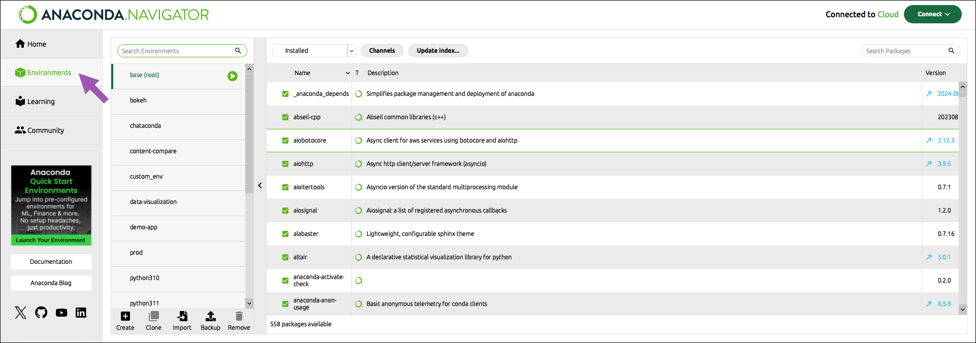 + 2. At the bottom of the environments list, click *Create*. - + 3. Select the python checkbox. @@ -50,7 +49,7 @@ Now that we have a clean environment configured, let us install some library we 1. Navigate to the environment page and select the environment we just created in the previous section. - + 2. Use the search bar in the top right corner to search for the following packages: @@ -74,6 +73,6 @@ From the *Home* page you can install applications, to the current environment we 3. From the Home page find the Spyder IDE tile. Click the *Install* button to start the download. - + 4. Once the download is complete, press *Launch* to start the applications.
\ No newline at end of file diff --git a/tutorials/module_1/spyder_getting_started.md b/tutorials/module_1/spyder_getting_started.md index ba055d7..c79568b 100644 --- a/tutorials/module_1/spyder_getting_started.md +++ b/tutorials/module_1/spyder_getting_started.md @@ -7,14 +7,14 @@ Using Anaconda we will select the environment we created earlier *spyder-dev* an ## Spyder Interface -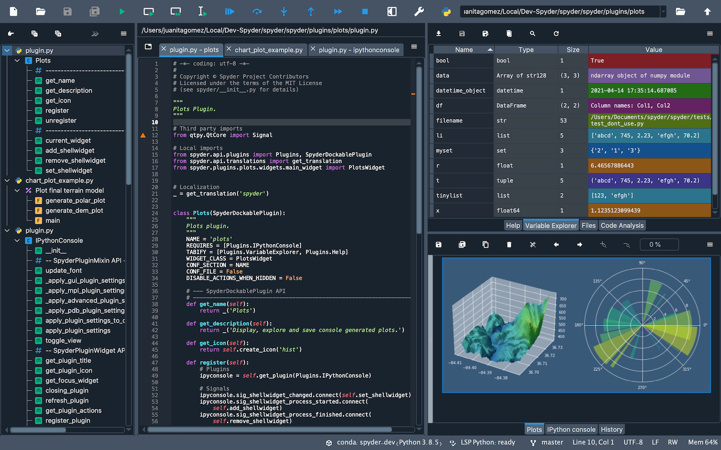 + Once you open up Spyder in it's default configuration, you'll see three sections; the editor IPython Console, Help viewer. You can customize the interface to suit your prefference and needs some of which include, rearrange, undock, hide panes. Feel free to set up Spyder as you like. ### Editor This pane is used to write your scripts. The -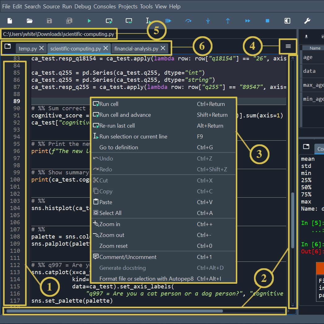 + 1. The left sidebar shows line numbers and displays any code analysis warnings that exist in the current file. Clicking a line number selects the text on that line, and clicking to the right of it sets a [breakpoint](https://docs.spyder-ide.org/5/panes/debugging.html#debugging-breakpoints). 2. The scrollbars allow vertical and horizontal navigation in a file. @@ -26,7 +26,7 @@ This pane is used to write your scripts. The ### IPython Console This pane allows you to interactively run functions, do math computations, assign and modify variables. -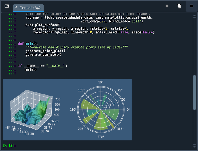 + - Automatic code completion - Real-time function calltips @@ -37,5 +37,5 @@ This pane allows you to interactively run functions, do math computations, assig ### Variable Explorer This pane shows all the defined variables (objects) stored. This can be used to identify the data type of variables, the size and inspect larger arrays. Double clicking the value cell opens up a window which allowing you to inspect the data in a spreadsheet like view. -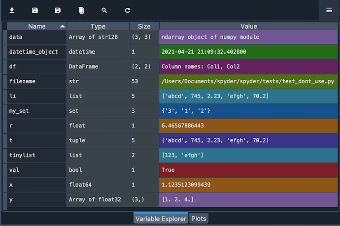 + |